B+ tree index

CSC 443

1. Overview of B+ tree

In the previous article, we discussed several important things about indexing:

Indexes are disk based data structures to speed up record search (and / or scan)
Organizing page pointers into sorted index tree structures speeds up record search. (ISAM)
Maintaining sortedness of the index tree is expensive, so we may create overflow pages in ISAM, but the overflow pages degrade search performance from $\log$ to linear scan.

We will introduce a highly robust and popular data structure B+ tree, which is an extension of ISAM.

Generally speaking, a B+ tree is an efficient disk based data structure that stores (key / value) pairs. It supports very efficient lookup by key, and iteration of entries in the range of two specified key values.

B+ tree offers:

fast record search
fast record traversal
maintaining sorted tree structure without overflow pages

The key idea behind B+ tree is that it utilizes balanced sorted tree of page pointers, as opposed to just sorted tree in the case of ISAM.

2. Definition of B+ tree

A B+ tree is a tree whose nodes are pages on disk. We will distinguish the leaf nodes and the interior nodes of a B+ tree.

Since each node is exactly one disk page, in the context of B+ tree, we use the term page and node interchangably.

2.1. Leaf nodes

The leaf nodes store the data entries in the form of (key, value). All leaf nodes are also organized into an linked list of pages. Leaf nodes of a B+ tree can be visualized as follows.

A leaf node

The following data structure abstracts the leaf nodes.

struct LeafNode {
    vector<Key> keys;
    vector<Value> values;
    PagePointer next_page;
}

We can always assert that

p.keys.size() == p.values.size() for all nodes p.

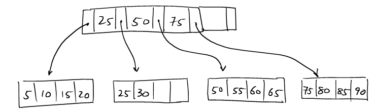
2.2. Interior nodes

The interior nodes form a tree structure, starting from a root node, to speed up lookup of the leaf node that contains a key of interest.

The structure of an interior node can be visualized as a sequence of alternating page pointers and keys.

An interior node

The following data structure abstracts the interior nodes:

struct InteriorNode {
    vector<Key> keys;
    vector<PagePointer> pointers;
}

We can always assert that p.keys.size() +1 == p.pointers.size().

Definition: Neighbouring pointers

Give a key $k_i$, we define $\mathrm{before}(k_i)$ to be the page pointer before $k_i$, and $\mathrm{after}(k_i)$ the page pointer after $k_i$.

Namely,

p.before($k_i$) = p.pointers[i]
p.after($k_i$) = p.pointers[i+1]

2.3. Constraints and properties of B+ tree

Keys are sorted in the nodes.

Let p be a node in B+ tree. We need to maintain that p.keys is sorted by the key values.

Nodes are sorted by their keys

B+ tree is a sorted tree in the following sense:

Leaf nodes are sorted:

$$ \forall p\in\mathrm{LeafNode},\; \forall k\in p.\mathrm{keys},\; \forall k'\in p.\mathtt{next\_page.keys},\; k \lt k' $$

The sorted linked list of leaf nodes allows very efficient traveral of (key, value) pairs between two leaf nodes.
Interior nodes are sorted:

B+ tree asserts that for all key $k$ and the adjacent pointers, $\mathrm{after}(k)$ and $\mathrm{after}(k)$, it must be that:
- $k \gt \max(\mathrm{keys}(\mathrm{before}(k))) $
- $k \leq \min(\mathrm{keys}(\mathrm{after}(k))) $
In other words, $k$ is the key that divides the keys in pages $\mathrm{before}(k)$ and $\mathrm{after}(k)$.

The tree is balanced

B+ tree is a balanced tree, so all paths from the root to the leaf nodes must be of equal length.

The nodes are sufficiently filled.

B+ tree permits nodes to be partially filled. As a design parameter, B+ tree specifies a percentage, known as the fill factor of the tree, that controls the minimal occupacity of all the non-root nodes.

If a non-root node is too empty, we say it has an underflow. Only the root node can have an underflow.

Here is an example of a problematic B+ tree. Suppose we have the following parameters:

    Capacity of each node: 4 keys
    Fill factor: 50%

While the tree is balanced and sorted, it does not satisfy the fill-factor.

‹›

3. B+ Tree Search and Insertion

The main operations on B+ tree are:

/**
 * finds the leaf node that _should_ contain the entry with the specified key
 */
LeafNode search(Node root, Key key)

/**
 * Inserts a key/val pair into the tree.
 * Returns the root of the new tree which _may_ be different
 * from the old root node.
 */
InteriorNode insert_into_tree(InteriorNode root, Key newkey, Value val)

The algorithm for insert must ensure that the properties of the B+ tree are preserved after the respective operation.

3.1. Searching

The B+ tree search algorithm is a straight-forward tree traveral algorithm.

LeafNode search(Node p, Key key) {
    if(p is LeafNode)
        return root;
    else {
        if(key < p.keys[0])
            return search(before(p.keys[0]), key);
        else if(key > p.keys[-1])
            return search(after(p.keys[-1]), key);
        else {
            let i be p.keys[i] <= key < p.keys[i+1]
            return search(after(p.keys[i]), key)
        }
    }
}

3.2. Inserting

Insertion into a B+ tree is quite tricky. Unlike the algorithm for insertion into a balanced sorted binary tree, the B+ tree insertion needs to deal with node overflows and underflows.

The insertion algorithm starts with:

look for the right leaf for insertion
try to insert into the leaf node

InteriorNode insert_into_tree(InteriorNode root, Key newkey, Value val) {
    LeafNode leaf = search(root, newkey);
    return insert_into_node(leaf, newkey, val);
}

The insertion algorithm, insert_into_node, looks something like this:

/**
 * Tries to inserts the (newkey/val) pair into
 * the node.
 *
 * If `target` is an interior node, then `val` must be a page pointer.
 */
InteriorNode insert_into_node(Node target, newkey, val) 
{
    if( ... CASE 1 ... ) {
        /* handle CASE 1 */
    } else if( ... CASE 2 ... ) {
        /* handle CASE 2 */
    } else if( ... CASE 3 ... ) {
        /* handle CASE 2 */
    }
}

The tree distinct cases are:

the target node has available space for one more key.
the target node is full, but its parent has space for one more key.
the target node and its parent are both full.

3.2.1. Case 1

This is the easiest case. Simply insert the entry (newkey, val) into target.

The root of the B+ tree does not change.
We have not discussed the disk I/O operations involved. Since all the node operations operate on one page at a time, the buffer manager can be used to provide the transparent virtual memory, as if all the nodes are stored in memory.

Example

(1): Suppose this is the initial tree. We are to insert (28, val) into this tree.

(2): Locating the insertion leaf target.

(3): Insertion complete.

‹›

3.2.2. Case 2

In this case, the target node is full, but its parent node has available space for at least one more key.

Create a new sibling node to target, call it new_target, and insert it after target.
Distribute the data entries between target and new_target. From the assumption that target is full, we can safely assert that after distribution, there will be no underflow.
new_target must be pointed to by (k,p) = (leaf2.keys[0], ADDRESS[leaf2]) in PARENT[target]. So (k,p) are to be inserted into PARENT[leaf]. By assumption, we know that PARENT[leaf] will not overflow.

Example

Let's continue with the previous example, and try to insert (70, val).

(1): We now insert an entry with key = 70.

(2): We locate the insertion leaf node, but it's full.

(3): We need to create new node and distribute the keys evenly.

(4): The new node creates a (Key, PagePointer) pair to be inserted into the parent.

(5): The parent has a vacancy, so (Key, PagePointer) can be simply inserted.

(6): Insertion of (70, val) completes.

‹›

3.2.3. Case 3

This is the case that both target and PARENT[target] are full. We have to recursively attempt to insert the new key into the ancestors of target. It is possible that even the root does not have sufficient space for the new key, in which case we must split the root, and create a new root node of the B+ tree.

The details are as follows:

Create new_target node, and insert it after target.
Distribute data entries among target and new_target.

Now, let k = leaf2.keys[0] and p = ADDRESS[leaf2]. We need to insert (k,p) into PARENT[leaf], which is full.

Let target_parent = PARENT[target]
Let all_keys = sorted(target_parent.keys $\cup$ {k})
Allocate new node new_interior
Let i = floor(all_keys.size() / 2).
Let middle_key = all_keys[i]
Distribute all_keys[0 .. i-1] to target_parent, and
Distribute all_keys[i+1 .. n] to new_interior.
If target_parent is the root, then let grandparent be a newly allocated node.
Otherwise, grandparent = PARENT[target_parent].
Recursively call:
insert_into_node(grandparent, middle_key, ADDRESS[new_interior])

Example

(1): We try to insert (95, ...) into this tree.

(2): The leaf node is full.

(3): As in CASE 2, we create a new leaf node and distribute the keys evenly.

(4): Here, the parent interior node is also full.

(5): We split the parent interior node, and distribute the keys before and after the middle key.

(6): The middle key is inserted to a new root node.

‹›

4. Other things about B+ Tree

B+ tree also offers efficient deletion. The deletion algorithm is a mirror reversal of the insertion algorithm. During deletion, the algorithm trys to merge nodes to avoid underflow. If a merge took place, deletion recursively deletes the (Key, PagePointer) pair from the parent node.
If the data entries are stored in a sequential file, sorted by a key, then one can very efficiently bulk load the sequential file into a B+ tree.
B+ tree can be used as a sorting algorithm for disk based sorting.